Specifying visual representations for model predictions and observed data using vmc • vmc

Introduction

This vignette describes how to use the vmc package to specify the visual representations used to describe the distribution of model predictions and observed data. We developed vmc to support visual representations of three types: area/extent, visual variable, and countable icon. For a more general introduction to vmc and its use on a standard model check workflow, see vignette("vmc").

Setup

The following libraries are required to run this vignette:

library(dplyr)
library(purrr)
library(vmc)
library(ggplot2)
library(ggdist)
library(cowplot)
library(rstan)
library(brms)
library(gganimate)
library(beeswarm)

theme_set(theme_tidybayes() + panel_border())

These options help Stan run faster:

rstan_options(auto_write = TRUE)
options(mc.cores = parallel::detectCores())

Model

We use the built-in model mpg_model, a brmsfit object fitted in Gaussian model family with push-forward transformations mu and sigma, to demonstrate different visual representations vmc defines to show the distribution of model predictions and observed data.

mpg_model
#>  Family: gaussian 
#>   Links: mu = identity; sigma = log 
#> Formula: mpg ~ disp + vs + am 
#>          sigma ~ vs + am
#>    Data: mtcars (Number of observations: 32) 
#>   Draws: 4 chains, each with iter = 6000; warmup = 3000; thin = 1;
#>          total post-warmup draws = 12000
#> 
#> Regression Coefficients:
#>                 Estimate Est.Error l-95% CI u-95% CI Rhat Bulk_ESS Tail_ESS
#> Intercept          23.25      2.87    17.57    28.92 1.00     6198     6420
#> sigma_Intercept     0.87      0.20     0.50     1.30 1.00    10336     7471
#> disp               -0.02      0.01    -0.04    -0.01 1.00     6404     6672
#> vs                  2.74      1.74    -0.73     6.14 1.00     6770     6991
#> am                  2.74      1.81    -0.76     6.36 1.00     6100     7119
#> sigma_vs            0.27      0.34    -0.38     0.95 1.00     6544     7801
#> sigma_am            0.34      0.36    -0.38     1.03 1.00     6925     7174
#> 
#> Draws were sampled using sampling(NUTS). For each parameter, Bulk_ESS
#> and Tail_ESS are effective sample size measures, and Rhat is the potential
#> scale reduction factor on split chains (at convergence, Rhat = 1).

Visualizing uncertainty using area/extent

vmc supports a list of visual representations to encode uncertainty using area/extent variable: - mc_model_slab() (mc_obs_slab()) - mc_model_ccdf() (mc_obs_ccdf()) - mc_model_cdf() (mc_obs_cdf()) - mc_model_eye() (mc_obs_eye()) - mc_model_halfeye() (mc_obs_halfeye()) - mc_model_histogram() (mc_obs_histogram()) - mc_model_pointinterval() (mc_obs_pointinterval()) - mc_model_interval() (mc_obs_interval()) - mc_model_lineribbbon() (mc_obs_lineribbon()) - mc_model_ribbon() (mc_obs_ribbon())

Examples:

mpg_model %>%
  mcplot() +
  mc_model_slab(alpha = .5) +
  mc_obs_slab(alpha = .5) +
  mc_gglayer(coord_flip())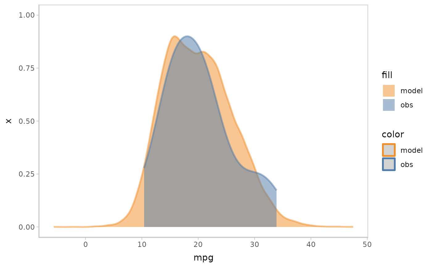

mpg_model %>%
  mcplot() +
  mc_model_slab(alpha = .5) +
  mc_obs_slab(alpha = .5) + 
  mc_condition_on(x = vars(vs)) +
  mc_gglayer(coord_flip())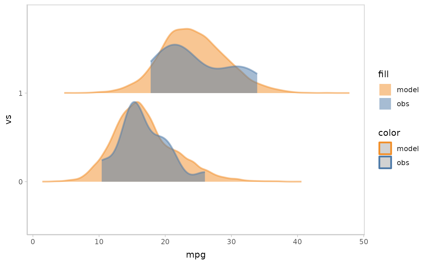

mpg_model %>%
  mcplot() +
  mc_model_slab(alpha = .5) +
  mc_obs_interval(alpha = .5) + 
  mc_condition_on(x = vars(vs)) +
  mc_gglayer(coord_flip())
#> Warning: Duplicated aesthetics after name standardisation: alpha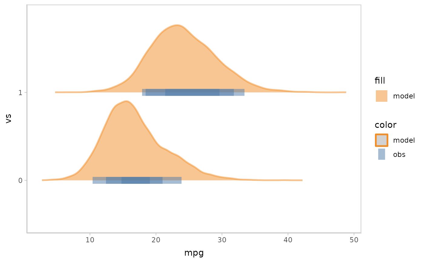

mpg_model %>%
  mcplot() +
  mc_model_lineribbon() +
  mc_obs_pointinterval() + 
  mc_condition_on(x = vars(disp))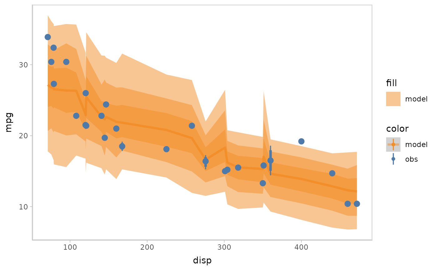

Visualizing uncertainty using visual variables

vmc supports a list of visual representation that encode uncertainty using diffferent visual variables: - mc_model_gradientinterval() (mc_obs_gradientinterval()) - mc_model_interval() (mc_obs_interval()) - mc_model_lineribbbon() (mc_obs_lineribbon()) - mc_model_ribbon() (mc_obs_ribbon()) - mc_model_tile() (mc_obs_tile())

Examples:

mpg_model %>%
  mcplot() +
  mc_model_gradientinterval() +
  mc_obs_point(shape = '|', size = 10) + 
  mc_condition_on(x = vars(vs)) +
  mc_gglayer(coord_flip())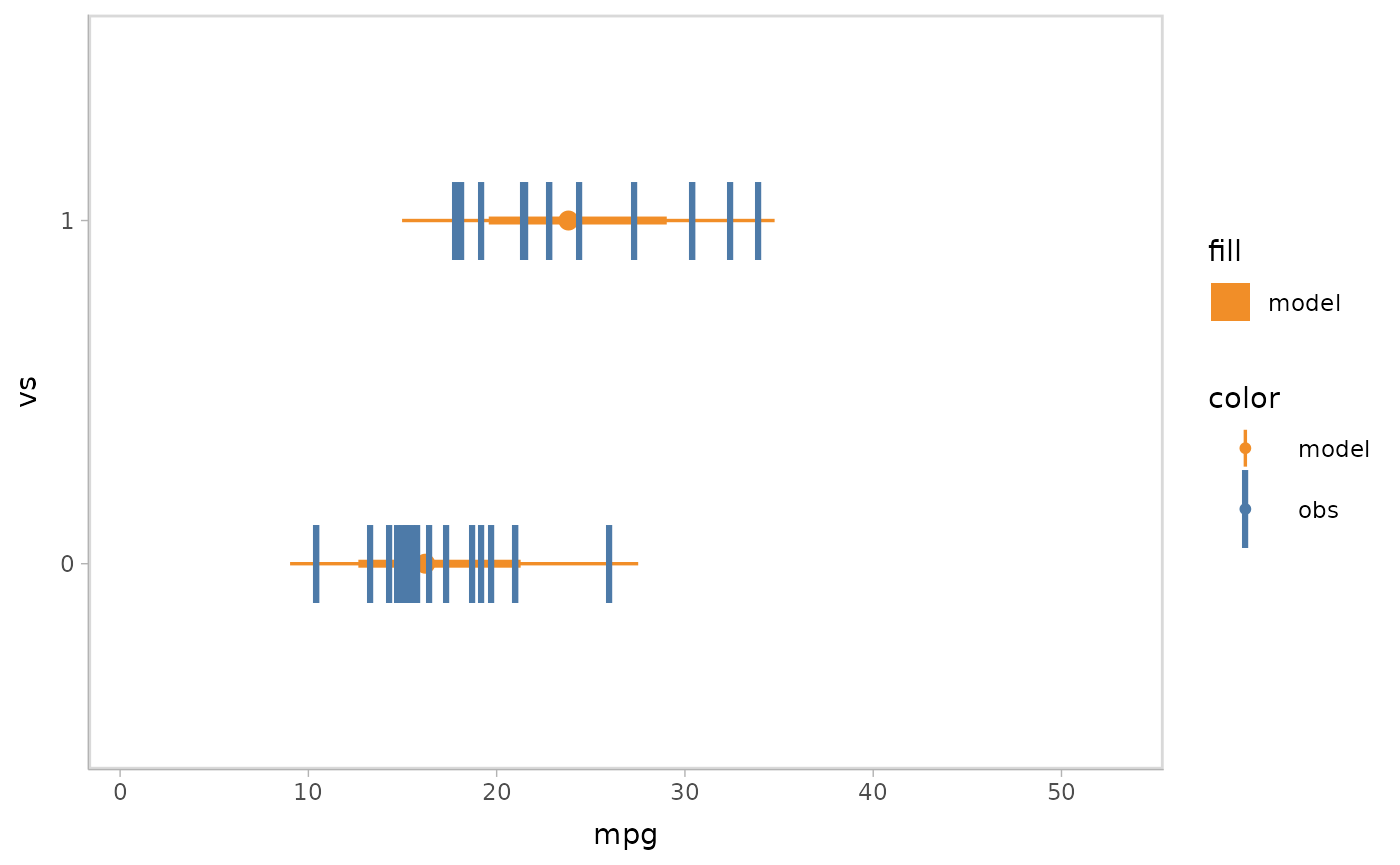

mpg_model %>%
  mcplot() +
  mc_model_gradientinterval() +
  mc_obs_gradientinterval() + 
  mc_condition_on(x = vars(vs)) +
  mc_layout_nested() +
  mc_gglayer(coord_flip())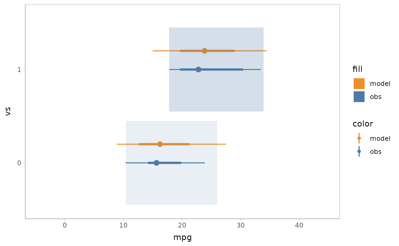

Visualizing uncertainty using countable icons

vmc supports a list of visual representations that encode uncertainty using countable icons: - mc_model_dots() (mc_obs_dots()) - mc_model_dotsinterval() (mc_obs_dotsinterval()) - mc_model_point() (mc_obs_point()) - mc_model_line() (mc_obs_line())

Examples:

mpg_model %>%
  mcplot() +
  mc_model_dots(n_sample = 100) +
  mc_obs_dots() + 
  mc_gglayer(coord_flip())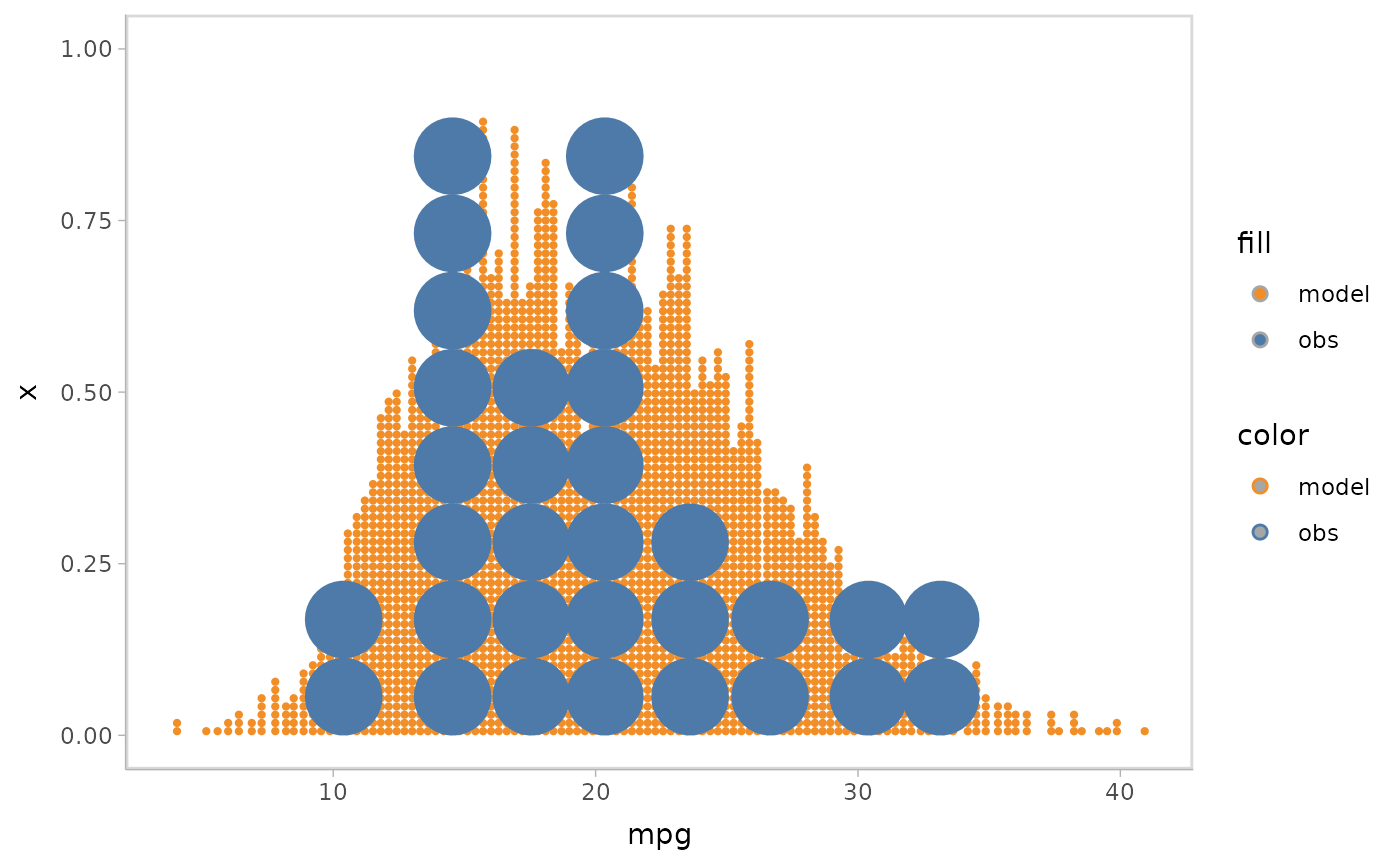

mpg_model %>%
  mcplot() +
  mc_model_slab() +
  mc_obs_interval() +
  mc_obs_dots(side = "left") + 
  mc_condition_on(x = vars(vs)) +
  mc_gglayer(coord_flip())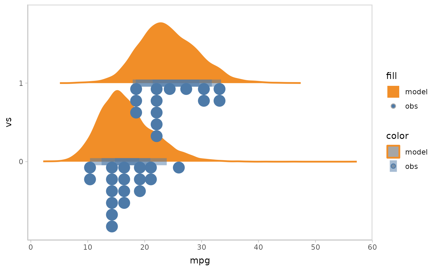

Customize the visual representation

If your visual representation is not supported directly by vmc, you can use mc_model_custom() and mc_obs_custom() to pass in a geom or stat function to specify the visual representation of model predictions and observed data. For example, we could use mc_model_custom(stat_boxplot) to specify a box plot for model predictions and mc_obs_custom(geom_swarm) to specify a swarm plot for observed data.

mpg_model %>%
  mcplot() +
  mc_model_custom(stat_boxplot, notch = TRUE) +
  mc_obs_custom(geom_swarm) +
  mc_condition_on(x = vars(vs)) +
  mc_gglayer(coord_flip())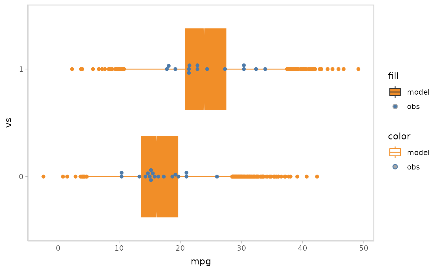

Grouping samples

vmc supports to show the uncertainty information conditioned on two sources, samples and input data points. Take the slab representation as example. In the beginning example, we are collapsing all the samples based on all the input data points together to form one distribution.

mpg_model %>%
  mcplot() +
  mc_model_slab(group_sample = "collapse") +
  mc_obs_slab() +
  mc_gglayer(coord_flip()) +
  mc_layout_juxtaposition()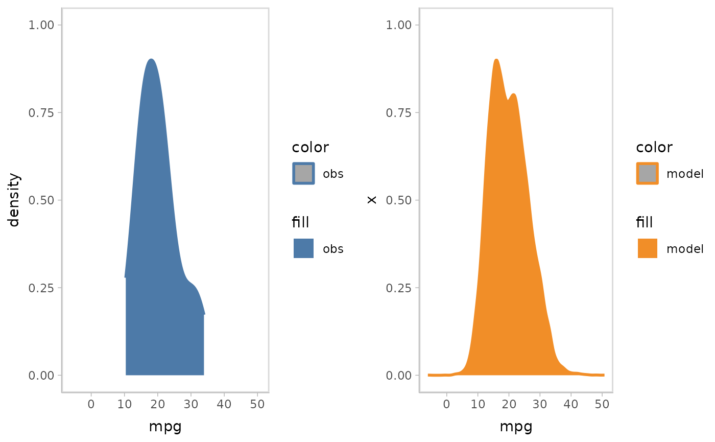

You can also choose to group by the sample when visualizing by slabs (i.e., using individual slabs for each sample).

mpg_model %>%
  mcplot() +
  mc_model_slab(group_sample = "group", alpha = .2) +
  mc_obs_slab() +
  mc_gglayer(coord_flip()) +
  mc_layout_juxtaposition()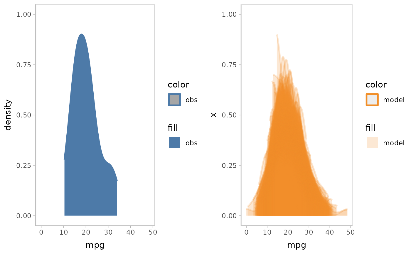

Or you can choose to group on input data point.

mpg_model %>%
  mcplot() +
  mc_model_slab(group_sample = "group", group_on = "row", alpha = .2) +
  mc_obs_slab() +
  mc_gglayer(coord_flip()) +
  mc_layout_juxtaposition()
#> Warning in layer_slabinterval(data = data, mapping = mapping, stat = StatSlab,
#> : Ignoring unknown parameters: `group_on`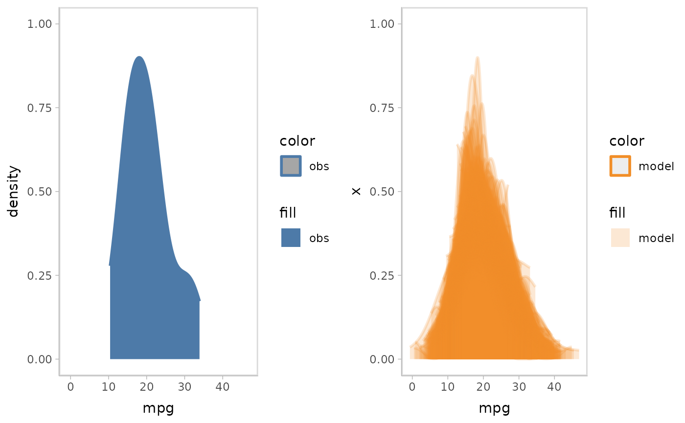

Instead of overlapping all samples or rows together, you can choose to use HOPs to show them each in one time frame.

mpg_model %>%
  mcplot() +
  mc_draw(ndraws = 50) +
  mc_model_slab(group_sample = "hops") +
  mc_obs_slab(alpha = .5) +
  mc_gglayer(coord_flip())
#> `nframes` and `fps` adjusted to match transition

You can also aggregate the model predictions from samples or input data points by functions.

mpg_model %>%
  mcplot() +
  mc_model_slab(group_sample = mean) +
  mc_obs_slab(alpha = .5) +
  mc_gglayer(coord_flip())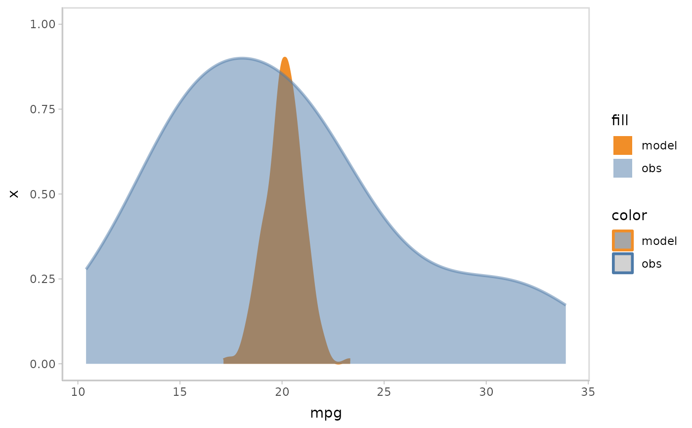

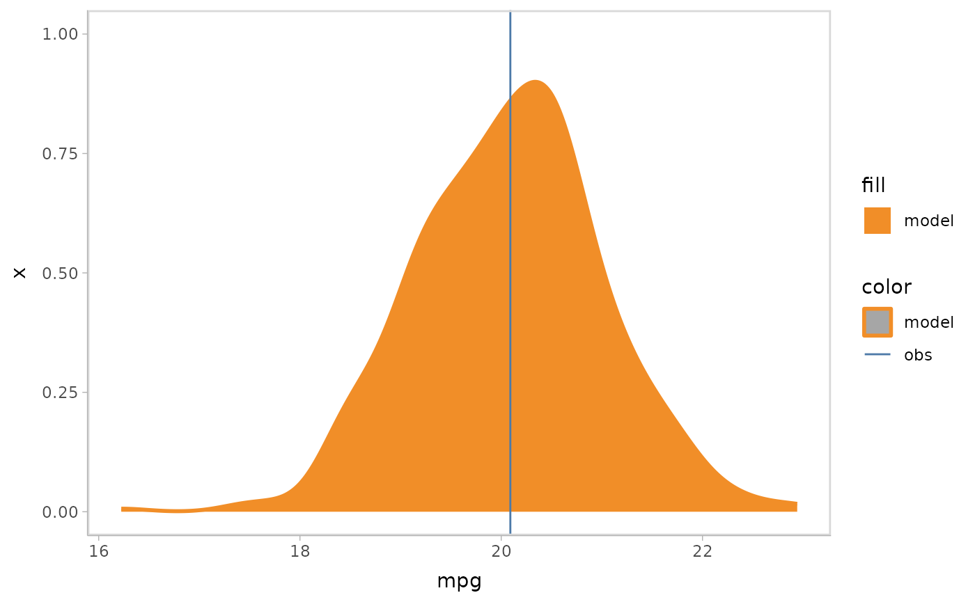
mpg_model %>%
  mcplot() +
  mc_observation_transformation(mean) +
  mc_model_slab(group_sample = mean, group_on = "row") +
  mc_obs_reference_line() +
  mc_gglayer(coord_flip())
#> Warning in layer_slabinterval(data = data, mapping = mapping, stat = StatSlab,
#> : Ignoring unknown parameters: `group_on`