Extracting arbitrary distributions from the model using vmc
distribution.RmdIntroduction
This vignette describes how to use the vmc package to
define how to extract a data frame to use in model checks (e.g., tidy
data frame) from arbitrary distributions that directly describe the
model predictions (e.g., posterior predictive distribution) or
indirectly describe the predictions via push-forward transformations
(e.g., model variables like mu and sigma in
Gaussian family models). For a more general introduction to
vmc and its use on a standard model check workflow, see
vignette("vmc").
Setup
The following libraries are required to run this vignette:
library(dplyr)
library(purrr)
library(vmc)
library(ggplot2)
library(ggdist)
library(cowplot)
library(rstan)
library(brms)
library(gganimate)
library(modelr)
library(insight)

theme_set(theme_tidybayes() + panel_border())
These options help Stan run faster:
rstan_options(auto_write = TRUE)
options(mc.cores = parallel::detectCores())
Bayesian models
vmc package uses the extraction functions from
tidybayes package, which can work for the Bayesian models
supporting fit and prediction, such as brms::brm() models
and rstanarm``](https://mc-stan.org/rstanarm/reference/rstanarm-package.html) models. For a full list of supported models bytidybayesextraction functions, see [tidybayes::tidybayes-models`.
We go through this section using a built-in model
mpg_model, a brmsfit object fitted in the
Gaussian model family with push-forward transformations mu
and sigma. The usage of other models is the same as long as
they are supported by the extraction functions from
tidybayes.
mpg_model
#>  Family: gaussian
#>   Links: mu = identity; sigma = log
#> Formula: mpg ~ disp + vs + am
#>          sigma ~ vs + am
#>    Data: mtcars (Number of observations: 32)
#>   Draws: 4 chains, each with iter = 6000; warmup = 3000; thin = 1;
#>          total post-warmup draws = 12000
#>
#> Regression Coefficients:
#>                 Estimate Est.Error l-95% CI u-95% CI Rhat Bulk_ESS Tail_ESS
#> Intercept          23.25      2.87    17.57    28.92 1.00     6198     6420
#> sigma_Intercept     0.87      0.20     0.50     1.30 1.00    10336     7471
#> disp               -0.02      0.01    -0.04    -0.01 1.00     6404     6672
#> vs                  2.74      1.74    -0.73     6.14 1.00     6770     6991
#> am                  2.74      1.81    -0.76     6.36 1.00     6100     7119
#> sigma_vs            0.27      0.34    -0.38     0.95 1.00     6544     7801
#> sigma_am            0.34      0.36    -0.38     1.03 1.00     6925     7174
#>
#> Draws were sampled using sampling(NUTS). For each parameter, Bulk_ESS
#> and Tail_ESS are effective sample size measures, and Rhat is the potential
#> scale reduction factor on split chains (at convergence, Rhat = 1).
Predictive distribution
Now we have the data ready for doing model check. We could use a
single mcplot() statement to generate a density plot for
predictive distributions, where vmc uses
tidybayes::predicted_draw() to extract tidy data frames
from the model and then compares it with the observed data that uses to
fit the model.
mpg_model %>%
  mcplot()
#> Warning: No shared levels found between `names(values)` of the manual scale and the
#> data's fill values.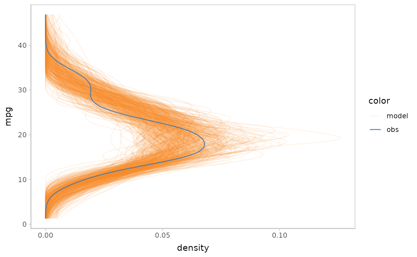
vmc puts the response variable on the y axis by default.
We could use ggplot2::coord_flip() to flip the axes.
mpg_model %>%
  mcplot() +
  mc_gglayer(coord_flip())
#> Warning: No shared levels found between `names(values)` of the manual scale and the
#> data's fill values.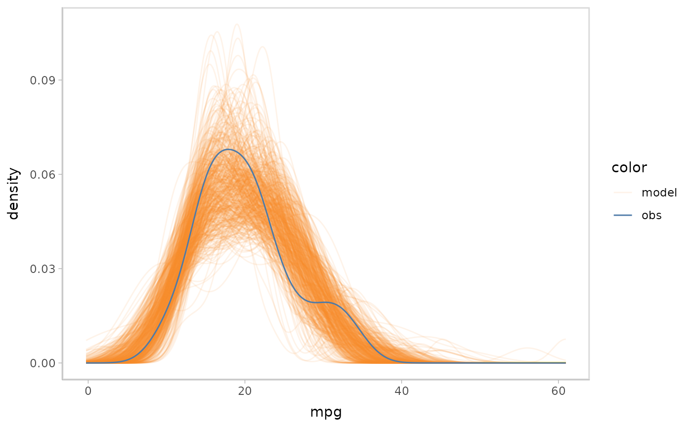
Push-forward transformations
Only checking the predictive distributions might not fulfill all the
purposes of model check. Imagine a scenario where the model designer
identifies misalignment between the model predictions and observed data.
This may lead them to want to know more details about which part of the
model leads it to behave differently from the observed data. For a
Bayesian model, they can access those quantities by extracting
push-forward transformations. For example, when they find a mismatched
pattern in a Gaussian predictive model, they can check whether the mean
of the model mismatches, the variance of the model mismatches, or
whether both mismatch by checking the mu push-forward
transformation and the sigma push-forward transformation
separately. After identifying which part is more responsible for they
discrepancy, they can correct that part in the formula of the model or
change the prior to better align predictions with the observed data.
mpg_model %>%
  mcplot() +
  mc_draw("mu") +
  mc_gglayer(coord_flip())
#> Warning: No shared levels found between `names(values)` of the manual scale and the
#> data's fill values.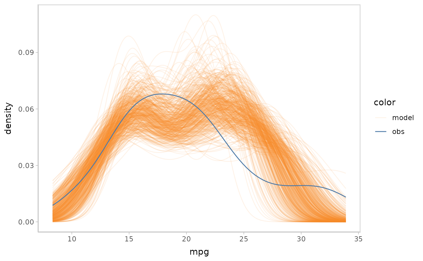
Some model variables have a different unit than the observations of
the response variable, such as sigma in a Gaussian model,
which will make them incomparable. In that case, we could add a
transform function for the observed data to bring them into the same
unit. For example, the sigma push-forward transformation
describes the variance of the observed data, so we could transform the
observed data using sd().
mpg_model %>%
  mcplot() +
  mc_observation_transformation(sd, vars(vs, am)) +
  mc_draw("sigma") +
  mc_gglayer(coord_flip())
#> Warning: No shared levels found between `names(values)` of the manual scale and the
#> data's fill values.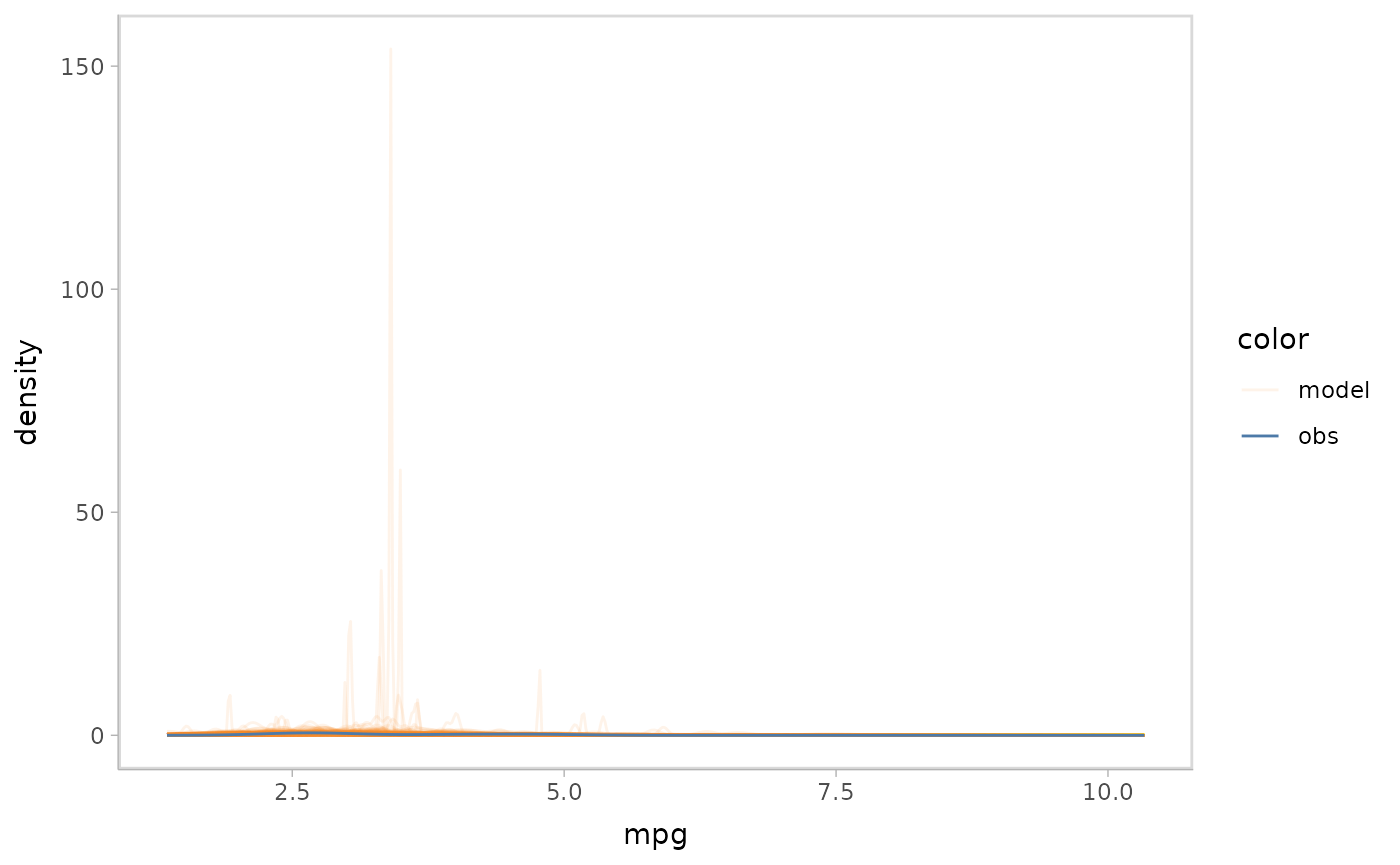
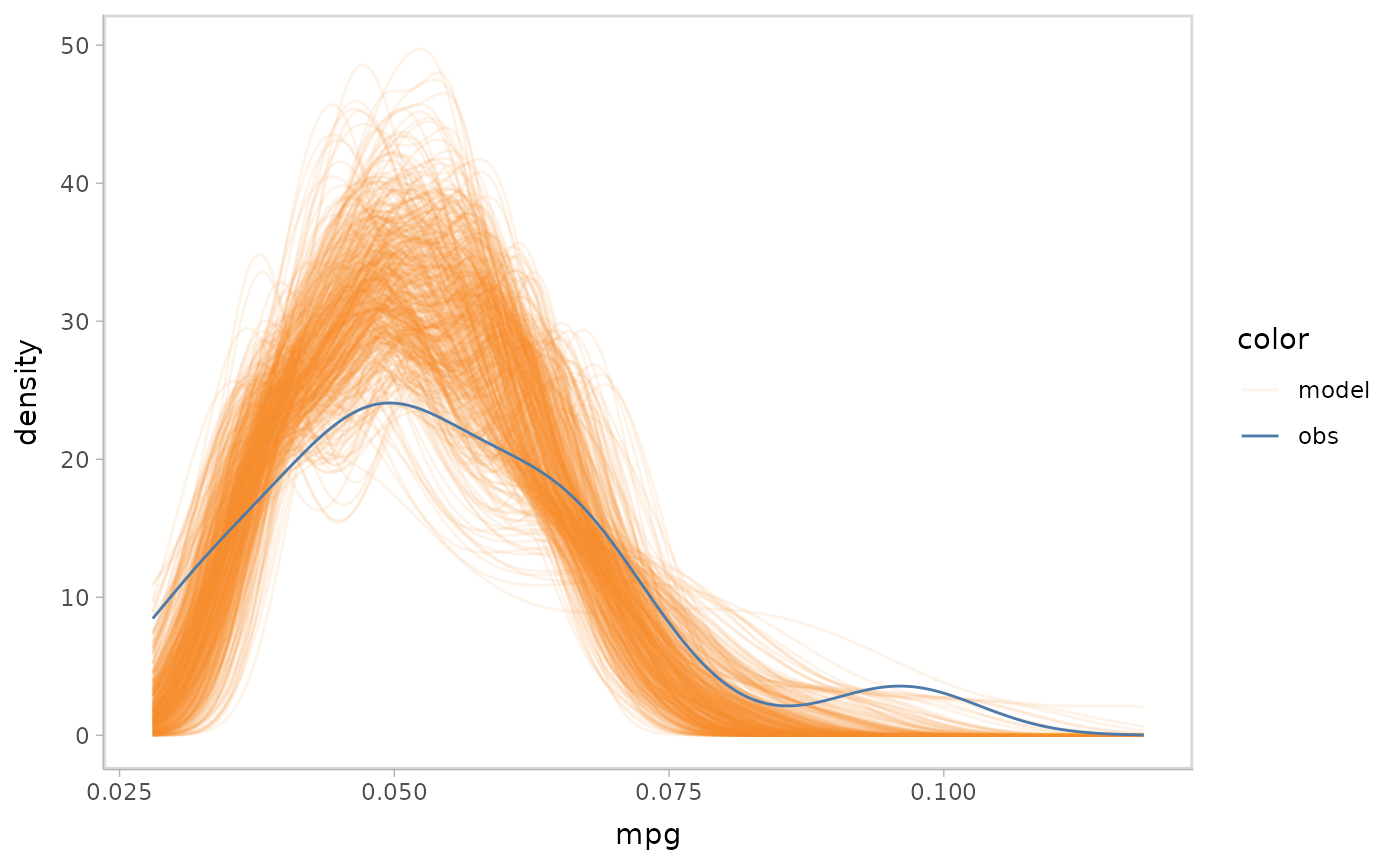
Note that we group the observation by vs and
am before transforming by sd() because the
model’s sigma has two predictors vs and am.
However you can also group them by other variables or even not group
them (which will make the observation a single value).
Distributions predicting on new data set
In a model check, we may want to generate the model’s prediction on a
new data set, rather than just replicating the output on the data that
is used to fit the model. For example, we may want to use
modelr::data_grid() to generate a grid describing the
predictors we want and then let the model predict on it.
mpg_model %>%
  mcplot() +
  mc_draw("prediction", newdata = data_grid(mpg_model$data, disp, vs, am)) +
  mc_gglayer(coord_flip())
#> Warning: No shared levels found between `names(values)` of the manual scale and the
#> data's fill values.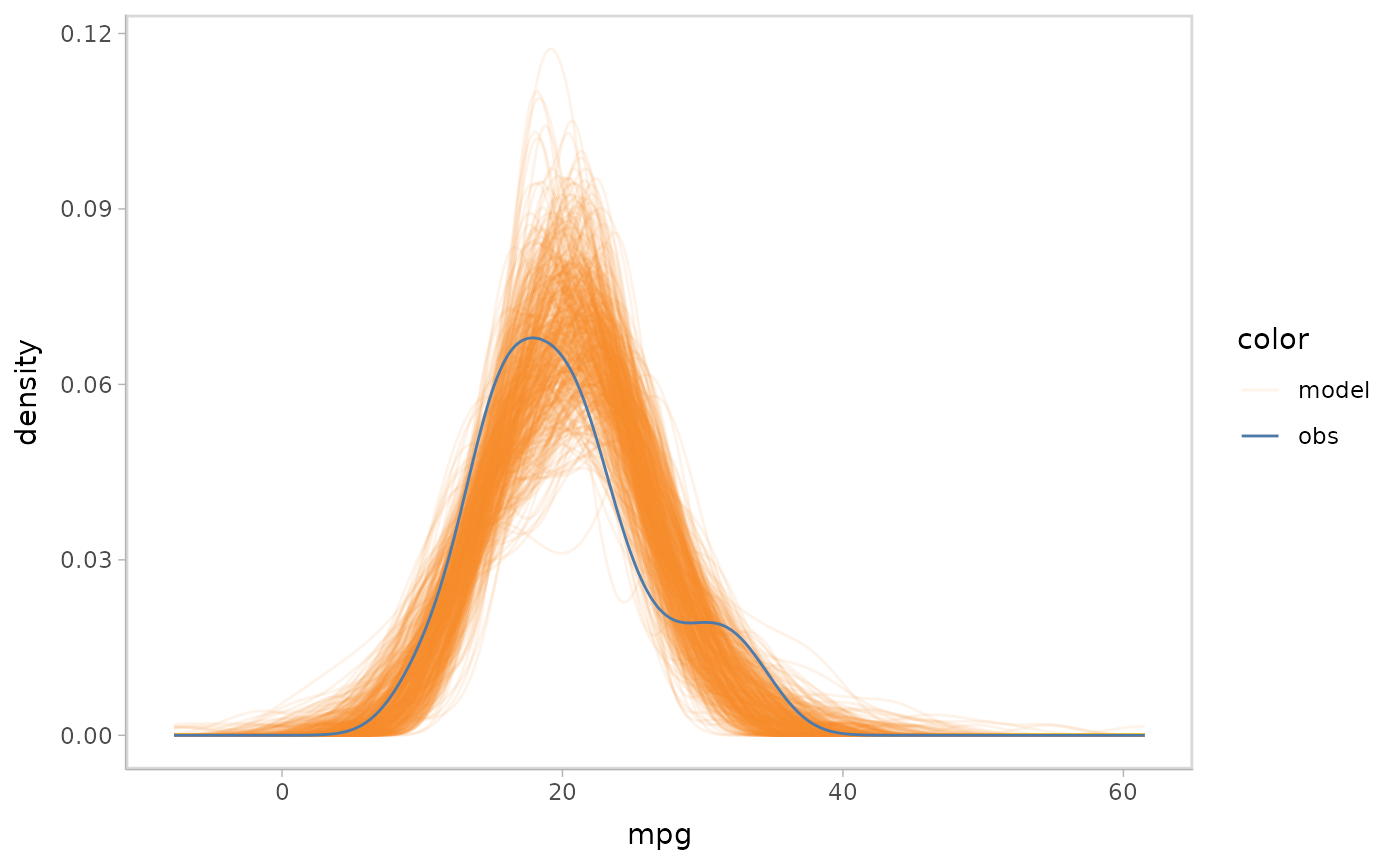
mpg_model %>%
  mcplot() +
  mc_draw("mu", newdata = data_grid(mpg_model$data, disp, vs, am)) +
  mc_gglayer(coord_flip())
#> Warning: No shared levels found between `names(values)` of the manual scale and the
#> data's fill values.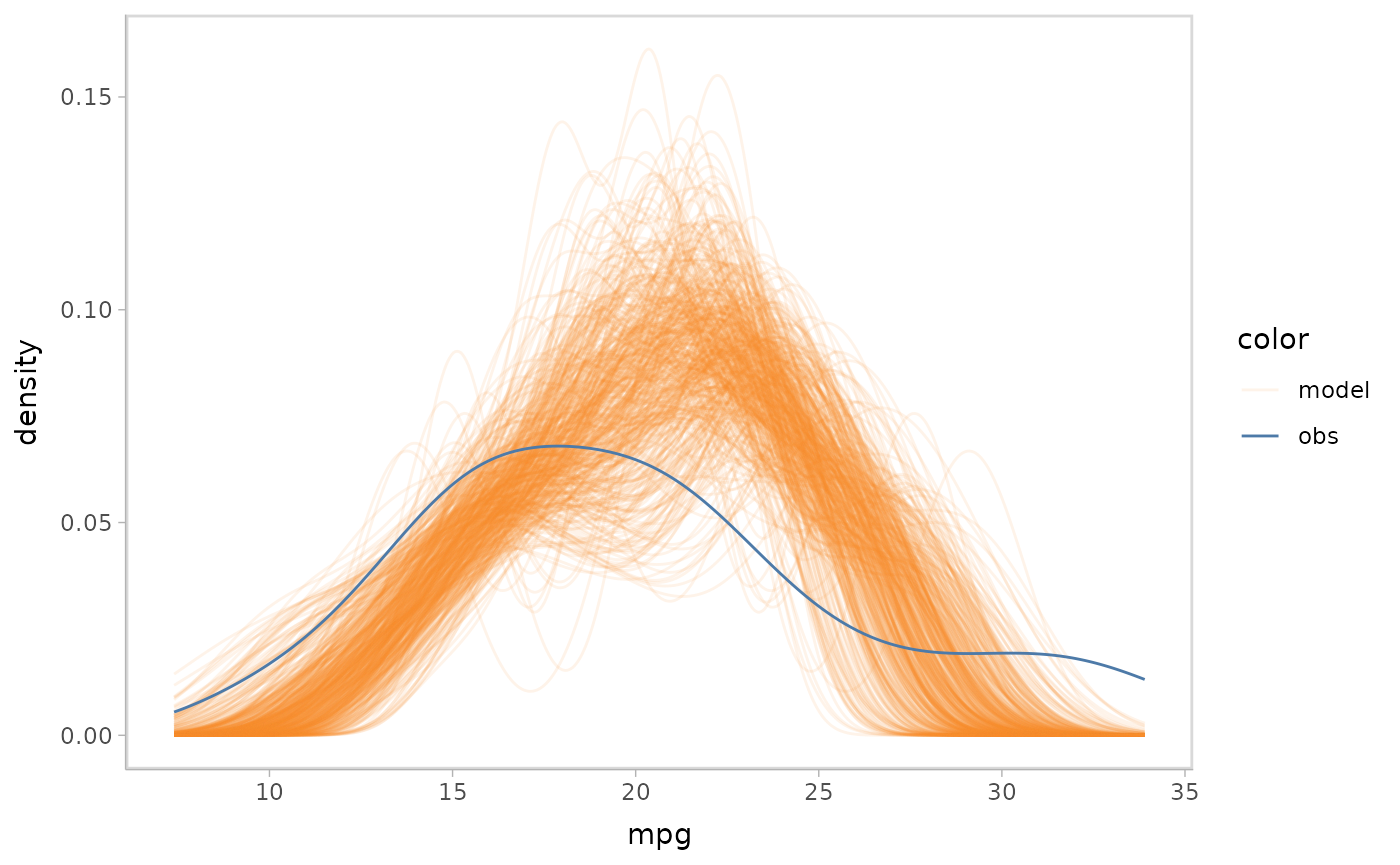
mpg_model %>%
  mcplot() +
  mc_observation_transformation(sd, vars(vs, am)) +
  mc_draw("sigma", newdata = data_grid(mpg_model$data, disp, vs, am)) +
  mc_gglayer(coord_flip())
#> Warning: No shared levels found between `names(values)` of the manual scale and the
#> data's fill values.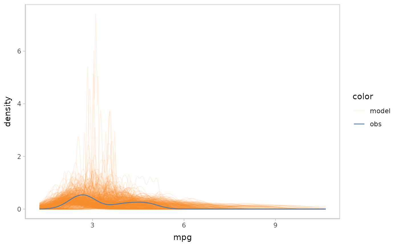
Frequentist models
For the models that are not supported by extract functions in
tidybayes, vmc uses
insight::get_predicted() to extract the distributions of
predictions and push-forward transformations. See a full list of the
model types supported by insight by
insight::supported_models(). We could choose these to show
the predictive distributions, link-scale distributions, and the
expectation distribution (the distribution of the expectation of the
predictions) when defining mc_draw().
We go through this section to show how to generate model checks using
vmc for an example general regression model that is fitted
using glm(family = "Gamma") with a push-forward
transformation on the inverse scale.
glm_model <- glm(mpg ~ cyl + hp, data = mtcars, family = "Gamma")
glm_model
#>
#> Call:  glm(formula = mpg ~ cyl + hp, family = "Gamma", data = mtcars)
#>
#> Coefficients:
#> (Intercept)          cyl           hp
#>   1.231e-02    4.618e-03    8.331e-05
#>
#> Degrees of Freedom: 31 Total (i.e. Null);  29 Residual
#> Null Deviance:       2.735
#> Residual Deviance: 0.6383    AIC: 162.9
Predictive distribution
Similar to Bayesian models, mcplot() generates a
predictive distribution from the model by default if no distribution is
specified.
glm_model %>%
  mcplot() +
  mc_gglayer(coord_flip())
#> Warning: No shared levels found between `names(values)` of the manual scale and the
#> data's fill values.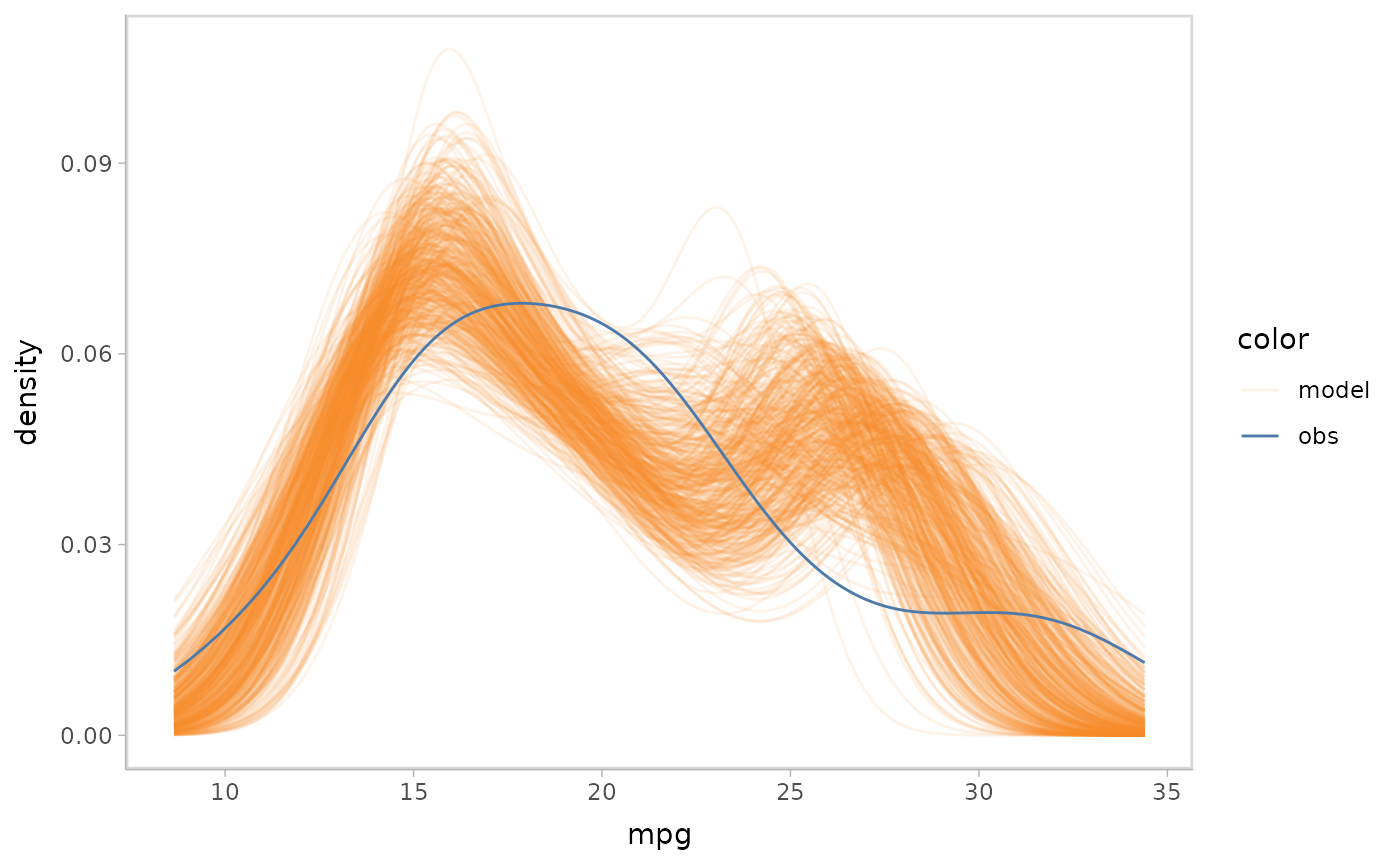
Push-forward transformations
The Gamma family in glm links the response variable
using inverse by default. Like the sigma push
forward transformation in the example Bayesian model, we could transform
the observed data into a scale that is comparable with the
inverse link in this model.
glm_model %>%
  mcplot() +
  mc_observation_transformation(function(x) 1/x) +
  mc_draw("link") +
  mc_gglayer(coord_flip())
#> Warning: No shared levels found between `names(values)` of the manual scale and the
#> data's fill values.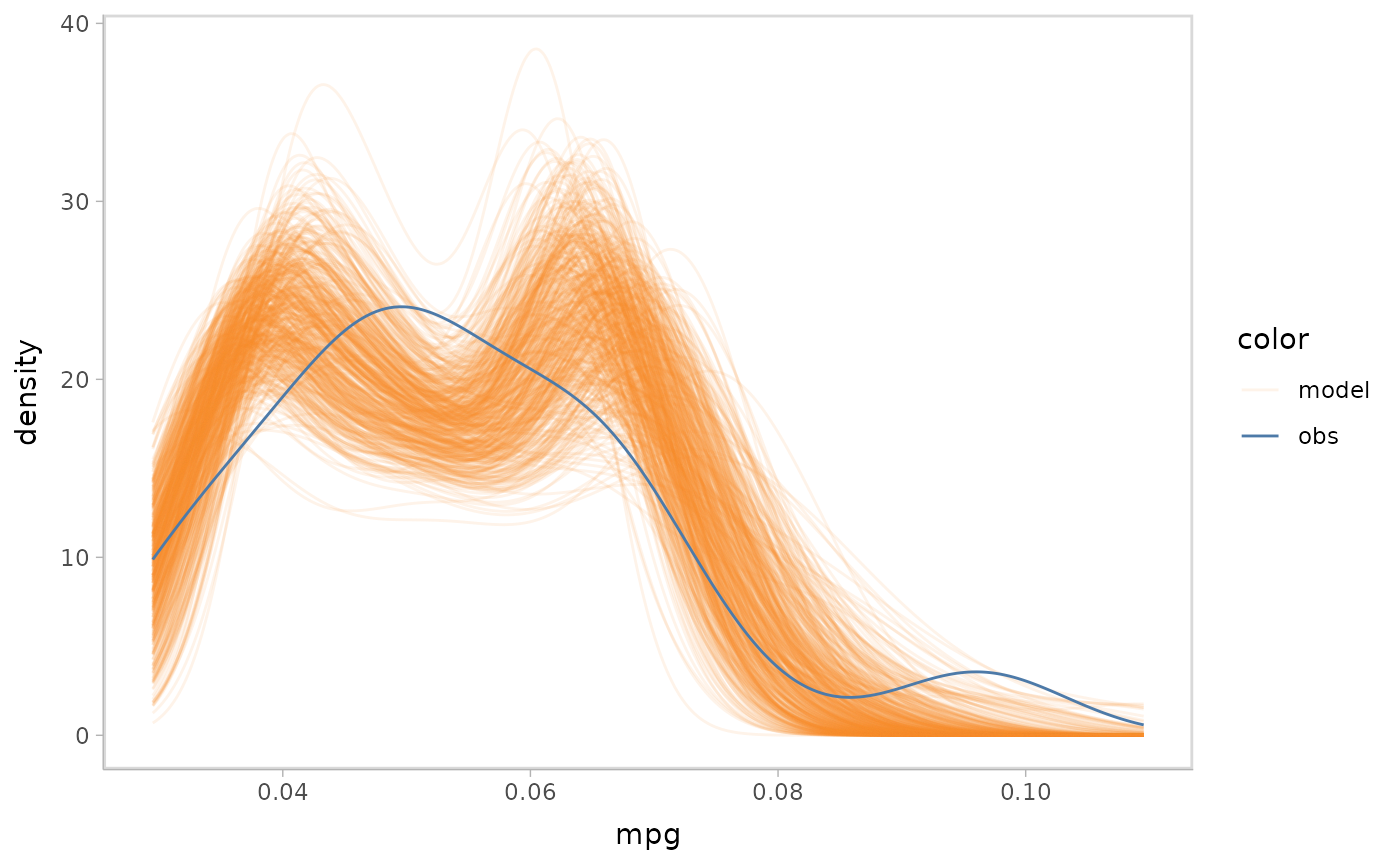
Distributions predicting on new data set
We could also specify a new data set to be used to generate distributions for non-Bayesian models.
glm_model %>%
  mcplot() +
  mc_draw("prediction", newdata = data_grid(get_data(glm_model), cyl, hp)) +
  mc_gglayer(coord_flip())
#> Warning: No shared levels found between `names(values)` of the manual scale and the
#> data's fill values.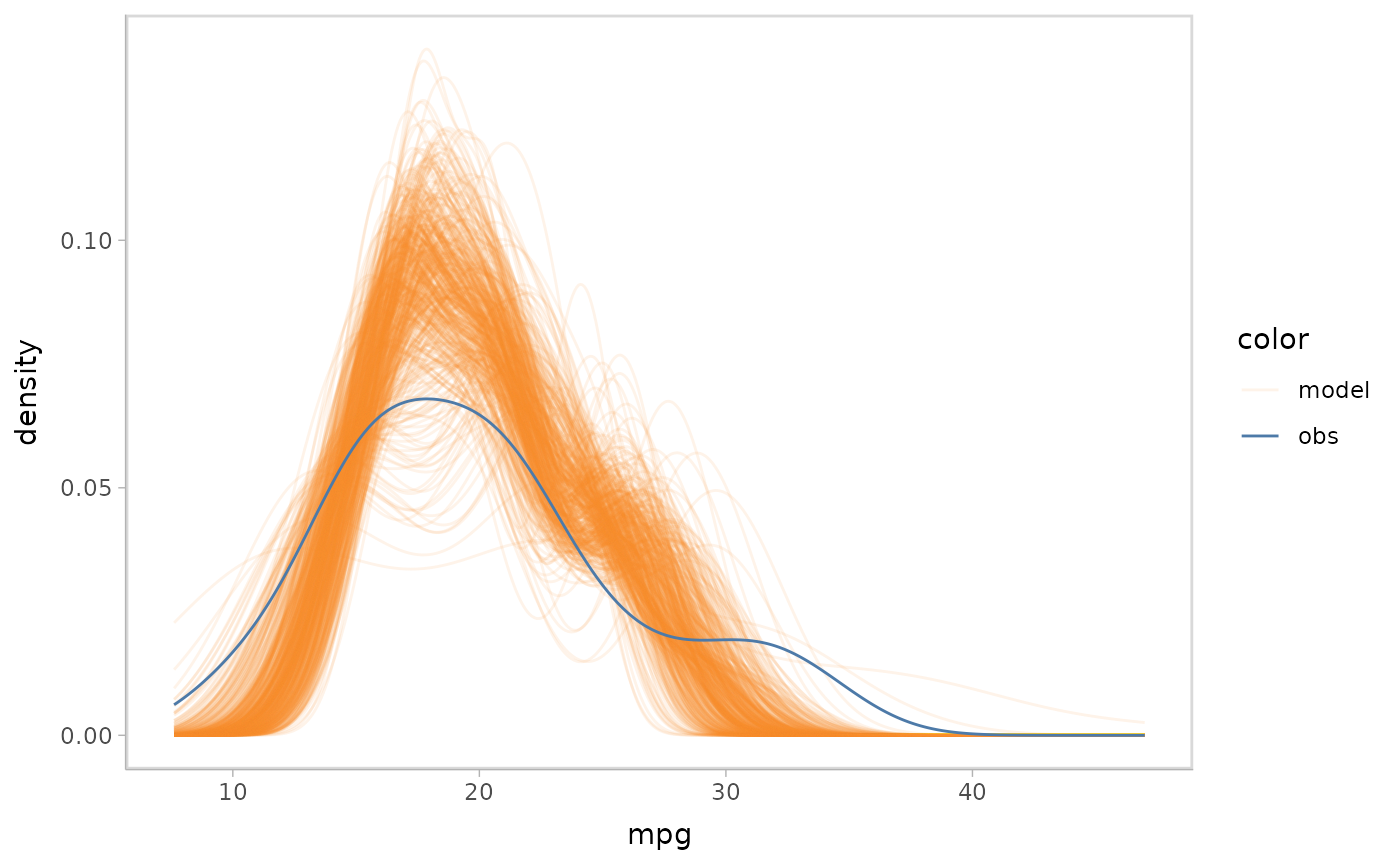
glm_model %>%
  mcplot() +
  mc_observation_transformation(function(x) 1/x) +
  mc_draw("link", newdata = data_grid(get_data(glm_model), cyl, hp)) +
  mc_gglayer(coord_flip())
#> Warning: No shared levels found between `names(values)` of the manual scale and the
#> data's fill values.