Comparing model predictions and observed data using vmc • vmc

Introduction

This vignette describes how to use the vmc package to specify a comparative layout that organizes the visual representation of model predictions and observed data into a layout to enhance visual comparison. We developed vmc to support comparative layouts of three types: juxtaposition, superposition, and explicit encoding. For a more general introduction to vmc and demonstration of its use in a standard model check workflow, see vignette("vmc").

Setup

The following libraries are required to run this vignette:

library(dplyr)
library(purrr)
library(vmc)
library(ggplot2)
library(ggdist)
library(cowplot)
library(rstan)
library(brms)
library(gganimate)

theme_set(theme_tidybayes() + panel_border())

These options help Stan run faster:

rstan_options(auto_write = TRUE)
options(mc.cores = parallel::detectCores())

Model

<<<<<<< HEAD We use the built-in model mpg_model, a brmsfit object fitted in Gaussian model family with push-forward transformations mu and sigma, to demonstrate different visual representations vmc defines to show the distributions in model and observed data. ======= We use the built-in model mpg_model, a brmsfit object fitted in Gaussian model family with checkable push-forward transformations mu and sigma, to demonstrate different visual representations that vmc defines to show the distributions of model predictions and observed data. >>>>>>> main

mpg_model
#>  Family: gaussian 
#>   Links: mu = identity; sigma = log 
#> Formula: mpg ~ disp + vs + am 
#>          sigma ~ vs + am
#>    Data: mtcars (Number of observations: 32) 
#>   Draws: 4 chains, each with iter = 6000; warmup = 3000; thin = 1;
#>          total post-warmup draws = 12000
#> 
#> Regression Coefficients:
#>                 Estimate Est.Error l-95% CI u-95% CI Rhat Bulk_ESS Tail_ESS
#> Intercept          23.25      2.87    17.57    28.92 1.00     6198     6420
#> sigma_Intercept     0.87      0.20     0.50     1.30 1.00    10336     7471
#> disp               -0.02      0.01    -0.04    -0.01 1.00     6404     6672
#> vs                  2.74      1.74    -0.73     6.14 1.00     6770     6991
#> am                  2.74      1.81    -0.76     6.36 1.00     6100     7119
#> sigma_vs            0.27      0.34    -0.38     0.95 1.00     6544     7801
#> sigma_am            0.34      0.36    -0.38     1.03 1.00     6925     7174
#> 
#> Draws were sampled using sampling(NUTS). For each parameter, Bulk_ESS
#> and Tail_ESS are effective sample size measures, and Rhat is the potential
#> scale reduction factor on split chains (at convergence, Rhat = 1).

Juxtaposition

Juxtaposition puts the visual representations of model predictions and observed data side by side. This comparative layout presents each object (visual representation for model predictions and observed data) separately, but requires that the viewer scan the plots to relate them. We specify the juxtaposition layout for a model check by mc_layout_juxtaposition().

mpg_model %>%
  mcplot() +
  mc_layout_juxtaposition() +
  mc_gglayer(coord_flip())
#> Warning: No shared levels found between `names(values)` of the manual scale and the
#> data's fill values.
#> No shared levels found between `names(values)` of the manual scale and the
#> data's fill values.
#> No shared levels found between `names(values)` of the manual scale and the
#> data's fill values.
#> No shared levels found between `names(values)` of the manual scale and the
#> data's fill values.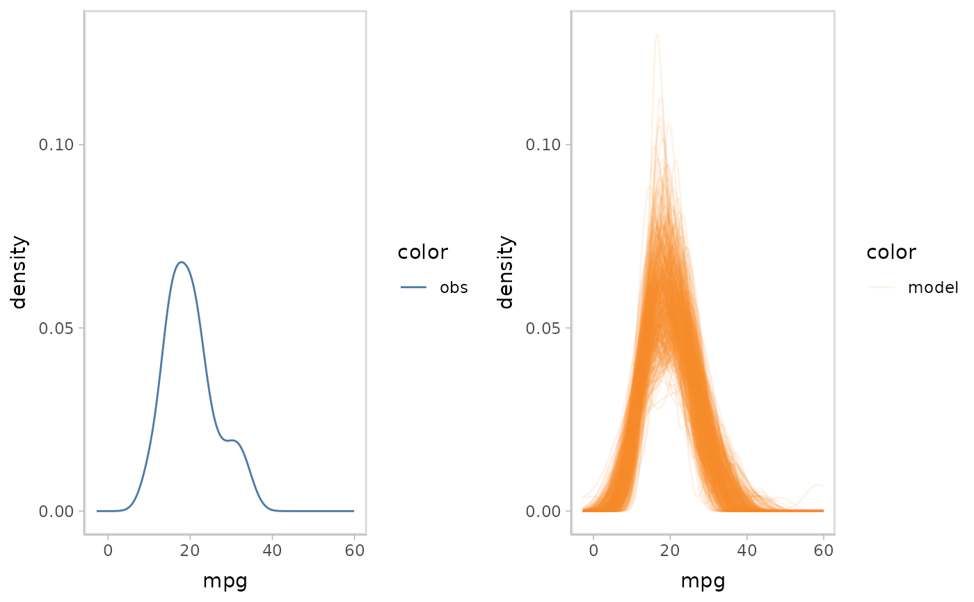

vmc also supports a variant of juxtaposition, nested juxtaposition, which helps reduce the amount of scanning required by viewers by nesting the juxtaposition layout in the plot when the model check has a discrete conditional variable. We specify this by mc_layout_nested().

mpg_model %>%
  mcplot() +
  mc_condition_on(x = vars(vs)) +
  mc_model_auto(n_sample = 1) +
  mc_layout_nested()
#> Warning: No shared levels found between `names(values)` of the manual scale and the
#> data's fill values.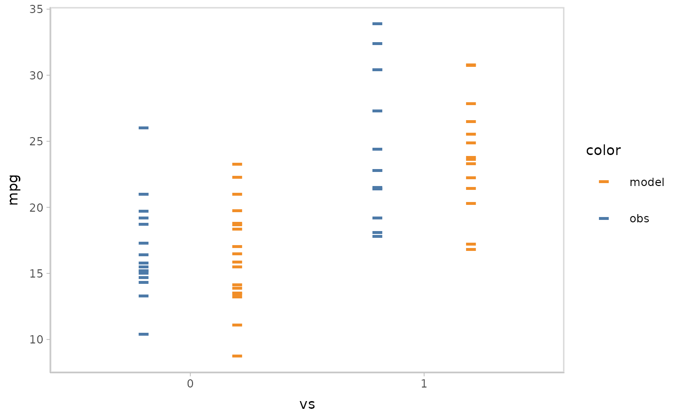

Superposition

Superposition overlays the objects (visual representations for model predictions and observed data) and presents the objects in a single coordinate system. vmc uses superposition as the default comparative layout if users don’t specify a comparative layout.

mpg_model %>%
  mcplot() +
  mc_layout_superposition() +
  mc_gglayer(coord_flip())
#> Warning: No shared levels found between `names(values)` of the manual scale and the
#> data's fill values.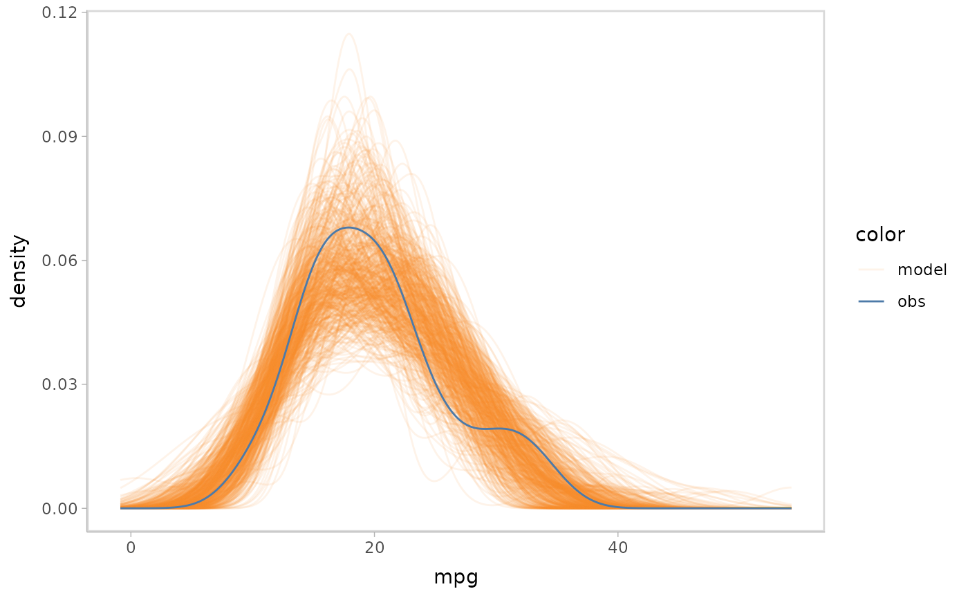

Explicit encoding

Explicit encoding directly encodes the connections between objects visually after calculating the difference between model predictions and observed data. For example, a residual plot presents the difference between the model predictions and observed data to encode the comparison about a central line encoding perfect prediction. A quantile-quantile (QQ) plot computes the quantiles of the residuals to encode the comparison.

Explicit encoding can also explicitly enable the user to check a model feature but not depends on viewer’s perception on the distribution of model prediction and observed data shown in raw coordinates of response variable and independent variables. For example, residual plot conditional on response variable enables to check linearity and QQ plot enables to check the normality of residuals.

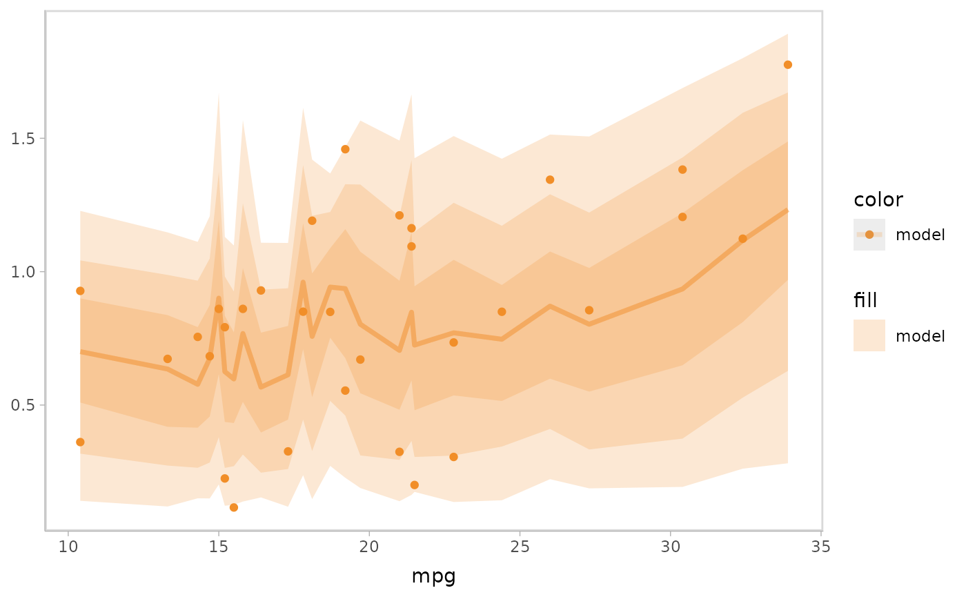
Let’s check the linearity of the model by specifying a residual plot conditional on the response variable mpg, where we use two visual representations (mc_model_lineribbon() and mc_model_point()) for the model predictions to reveal the trend of residuals while also showing a set of raw data points.

mpg_model %>% 
  mcplot() + 
  mc_condition_on(x = vars(mpg)) + 
  mc_layout_encoding("residual") + 
  mc_model_lineribbon(alpha = .2) + 
  mc_model_point(n_sample = 1) + 
  mc_gglayer(geom_hline(yintercept = 0))
#> Warning: Duplicated aesthetics after name standardisation: alpha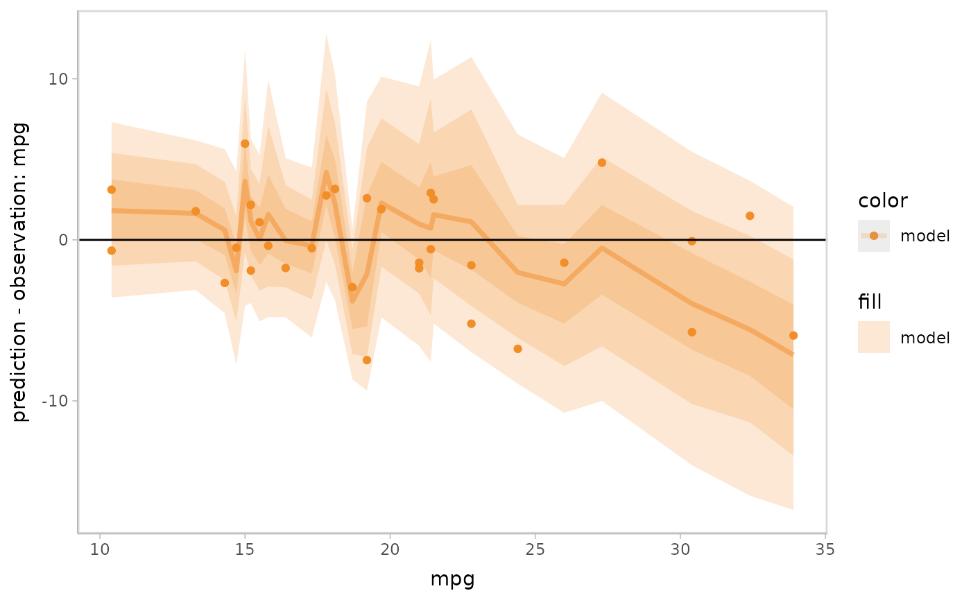

Next let’s check the normality of the residuals by drawing a QQ plot. We could specify this easily by using mc_layout_encoding(tranform = "qq").

mpg_model %>% 
  mcplot() + 
  mc_layout_encoding("qq") + 
  mc_model_point(n_sample = 1) + 
  mc_gglayer(geom_abline())
#> Warning: No shared levels found between `names(values)` of the manual scale and the
#> data's fill values.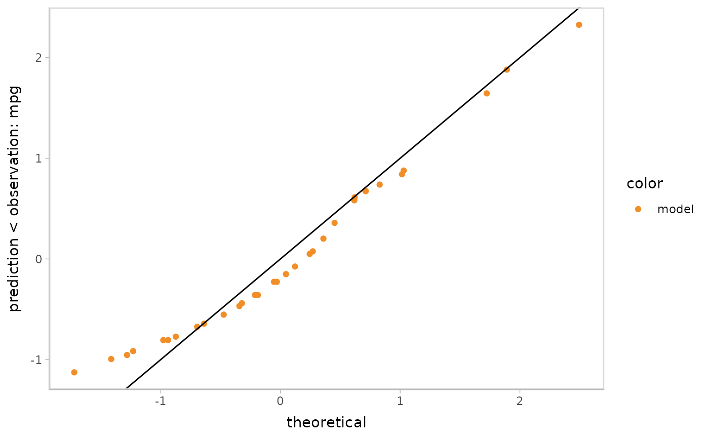

Specify your own explicit encoding

We could use vmc to specify a customized transformation function that computes the comparison between model predictions and observed data. The transformation function should take as input a data frame that is generated from the newdata data frame in mc_draw() (if not specified, it’s the data used to fit the model, e.g., you can get that by insight::get_data(model)) with additional columns: .row, .draw, prediction, and observation (if newdata has a column for the response variable). We can transform the input data frame to generate a new one that has the columns for the variable shown on the y-axis and x-axis named as y_axis and x_axis (optional).

Here is an example of a customized explicit encoding, where we want to check the variance of residuals.

var_res_func = function(data) {
  data %>%
    mutate(y_axis = prediction - observation) %>%
    mutate(y_axis = sqrt(abs(y_axis / sd(y_axis))))
}

mpg_model %>% 
  mcplot() + 
  mc_condition_on(x = vars(mpg)) + 
  mc_layout_encoding(var_res_func) + 
  mc_model_lineribbon(alpha = .2) + 
  mc_model_point(n_sample = 1)
#> Warning: Duplicated aesthetics after name standardisation: alpha